Home Artwork Page Comp Art Page Books Calenders Food and Brew Page Metal Working Page Links Page Pictures Page Projects Page CAFL Control Algorithm DOS Bootsector DFP Project Linux Page Music Page Recursive Logistic Eqn RF Electronics Projects Software Projects Temperature Data Logging Wind Chime Weather Page

This projects page contains some software projects, some were written in compiled BASIC others in C. Others without an in depth description appear in a Software Portfolio listing. The source code is available via FTP at ftp://ftp.frontiernet.net/pub/users/erickclasen/public_ftp/C/ and ftp://ftp.frontiernet.net/pub/users/erickclasen/public_ftp/BAS/ respectively for C files or BASIC files. Most of them are simple command line utilities, however a few are quite complex. The BASIC programs I compile with the Power Basic compiler. The C programs are compiled with Borland 3.0 or GCC depending on the target. Data Encryption Program Basic description of data encryption. Lunar Phase Program Creates an almanac of moon and sun positions. Weather Statistics Program Approximate sunrise and sunset, average temperatures for a given day. Command Line Calculator Program A very simple calculator that works directly from the DOS command line. Cellular Automata Graphics Programs Draws various cellular Automata on the screen. CAT Transceiver Control Program Controls a Yaseu FT767GX HF Transceiver using a PC via the serial port.   First a bit of history When I started with computers in 6th grade it was with a TRS-80 pocket computer (Clock speed 540 kHz, ~1K RAM), the first version that they sold. This was followed quickly by a VIC-20 (6502@2mHz, 3K RAM). As I got used to BASIC, I started writing more and more complicated programs. Some favorite non-graphical games were a stock market game based on random prices attached to letter sequences that were generated. From the initial price, small random deltas were introduced to the prices. The object of the game was to watch the "ticker tape" ASCII go by on the screen and buy and sell the stocks, making a profit. This was sort of a day trading game, simple but entertaining. Another was a non-graphical flight simulator that was based on some basic physics, using numerical methods. On the screen you would see the instruments represented in numbers and would fly based on these instruments. A lot of work was put into this one and it worked fairly good for what it was. The next big step was graphics, most programs written with graphics were a hybrid, BASIC for the main program with machine language calls for the graphics routines. One of the initial hurdles was the fact that there was no assembler available at the time for the VIC-20. I wrote a few short segments of machine language by poking in the op-codes using the 6502 book, this got old fast. But it did prove the merits of machine code. The speed difference was amazing. Filling the screen entirely with one repeated character would take a noticeable amount of time in BASIC. Using machine code, it would appear to instantly flash the entire screen at once. I was hooked. I then wrote an assembler/machine language monitor tool in BASIC using the 6502 book as a guide. This enabled me to write in assembly and load the machine code into memory. This worked better, still slow going to write software. But the payoff was that the machine language could write to the screen at a much higher rate that the interpreted BASIC. The easiest way to load the assembly was to treat it as data and allow the BASIC program to load it into RAM on start up. This made it possible to write games that had a lot of graphics refresh such as Pacman and grotto style games. Besides writing game software I wrote some software that would model physics such as simulations of launching artillery and missiles. One other thing I used frequently and toyed with was numerical methods. I was basically doing calculus type math on the computer, years before I knew what it was. One of my favorites at that time was algorithms along the lines of Newton's method. Newton's method is typically used to find a square root by successive approximations. I used it and an algorithm that closes in on a target value using a Tractrix curve in a lot of places. These were used as control algorithms behind the flight simulator and controlling the ghosts on the Pacman game. That sums up how I started with programming.   Data Encryption of Files Using Random Files as Keys The concept used is to take 2 files reading them in as binary data, and applying a mathematical operation between them. The key file must be at least as long as the file to be encrypted. Preferably the key file would be created by a random number generator. Simplistically the encode operation could just add the 2 files byte wise and simply allowing rollover to occur. The decode operation would then subtract the characters of the key file back out from the encrypted file. The following shows an example of encrypting the word hello. Add Method Input File Key File Output File Letter ASCII ASCII value value value h 104 63 203 e 101 87 188 l 108 135 243 l 108 68 176 o 111 222 77 (111+222 = 333 with '8 bit rollover' 333-256 = 77) To decode the output file requires the key file and works by subtraction. Subtract Decryption Input File Key File Output File ASCII ASCII ASCII Letter value value value 203 63 104 h 188 87 101 e 243 135 108 l 176 68 108 l 77 222 111 o (77-222 = -145 with '8 bit rollover' -145+256 = 111 ) The previous description requires 2 programs. One to encrypt and another to decrypt. A way to make decryption and encryption work with one program is to make it a mirrored process. Instead of adding for encryption and subtracting for decryption using an operation such as a logical XOR (exclusive or) would accomplish the mirroring process. In electromechanical cryptography (i.e. Enigma machine) this would be a reflector operation. The encode operation would appear as follows. XOR Method Input File Key File Output File Letter ASCII ASCII ASCII value value value h 104 63 87 e 101 87 50 l 108 135 235 l 108 68 40 o 111 222 177 To decode the output file requires the key file and works by subtraction. XOR Decryption Input File Key File Output File ASCII ASCII ASCII Letter value value value 87 63 104 h 50 87 101 e 235 135 108 l 40 68 108 l 177 222 111 o (77-222 = -145 with '8 bit rollover' -145+256 = 111 ) The result is that the same algorithm and program can be used both ways in the XOR case. The weakness in both the add-subtract and the XOR method is that using a key of zero allows the character to be sent to the output file unencrypted. If this happens intermittently only a few instances per message it is OK. If it happens to often it may be possible to decode the file using a frequency analysis attack. The object in any type of encryption is to completely mix the message with the key. This mix should make the output as random as possible. The frequency table of the output should be as close to white noise as possible. The key should be large enough that it does not repeat within the message. If the key does not have enough combinations in it so that a pattern forms, as in it repeats after some number of bytes then it is not a good key. By having a pattern in a key, there is a possibility of attack on the encrypted data by detection of this pattern and working backwards from it. The best key and in the case of using a file as a key, the best file would be a file of white noise. Pseudo-random number generators suffer from the problem that they are generated using an algorithm themselves. This leads to the problem that eventually the key may repeat. If the key repeats after n characters and the message/file that is to be encrypted is less than n no problem, if not the key is weak. Another problem with pseudo-random number generators is the fact that they require a seed value. They are a finite number of seed values, for a given seed value the sequence of pseudo-random numbers will be the same. Generally the programmer tries to use tricks like reading a clock and a piece of memory like a register that can have any sort of data in it at that time. But the fact remains that the same seed with generate the same key sequence. If you encrypt enough files and messages eventually over time two of them will be using the same key. This lends itself to cracking the code by pattern matching between files/messages. This pattern matching to crack codes can get elaborate and use common English works as tries against the patterns. These so called cribs provide shortcuts to cracking codes. For instance it could be assumed that a message from John to Sue will contain Sue in the message, not mention words like (the) and (and). This fact can be used in combination with pattern matching, looking for messages or segments of messages encoded with the same key sequence. The best random numbers to use as a key and create a key file from would be true random numbers. Random number generators that work by use Johnson (thermal) noise as there source would be the best. It is possible to generate such a source by using Zener diode noise fed into an A to D converter. That would allow getting a digital value for the noise, best would be to have it mapped to a memory location where it can be easily read. This number then could be read to the key file, generating a truly random key. This could even be done using the microphone input on a computer. By connecting a noise source to the microphone input and generating a WAV file from it, this file can be used as the random key with which to encode the message. This is just a small simple (although very effective) example and taste of cryptography. Other information can be read on-line about it. The history of the Enigma machine and decoding it in project Ultra is interesting in particular. There is something called public key encryption, so called PGP is an example. This is worth looking at as well. Books Here????? Back to Top   Lunar Phase Program The almanac and calender information presented on the Almanac with Sun and Moon Position and Lunar Events pages was generated by a software algorithm. It is quite accurate, so far it seems to line up well with the reality in the sky. For the lunar months, the numbering was considered to start with the first new moon of the new calender year, this is somewhat arbitrary and there might be some better suggestions. The time base for the calculations is UTC. Items calculated for a given day are calculated at 00:00 UTC for that day. The moon Zodiac gives the moons position exactly when it is in a given sign. The sun Zodiac follows the traditional, divide the year up into 12 equal parts method. Glossary of abbreviations AGE = Moons age in days since it became new. D(AU) = The suns distance from the earth, in Astronomical Units. D(ER) = The moons distance in Earth radii. Exct Zodiac = Zodiac that the moon is in, exactly, no rounding to a 30 degree window. LAT = The moons latitude along the ecliptic, in degrees. LONG or Mn LONG = The moons longitude along the ecliptic, in degrees. MM/DD/YYYY:HH:MM = Format in date and 24 Hour time UTC. Sun Age = The number of days since the last spring equinox. Sun LAT = The Suns latitude along the ecliptic, in degrees. Sun LONG= The approximate position of the Sun in degrees latitude with reference to the earths equator. The software was built in C some of the parts of the code namely the algorithms for the moon and sun position were available on-line from observatories. SAAO- NAO Technical Note No. 46(1978) and Moonlight Cascade Observatory/BBS. Around the algorithms an interface was built that drives the program from the command line. I consider the data to be accurate, but there are no guarantees as with any software. Code was then created to format the output. Tables in the code was created, for example one to interpret the Zodiac sign correctly, deriving the zodiac given the ecliptic longitude. Internal to the program the date that is input by the user is converted to Julian date. The program is aware of the switch over from Julian to Gregorian calender and accommodates this as well. The Gregorian calender fix is to, force a date in the range 10/4 - 10/14/1582 to 10/15/1582. This forces the values in range, being that the calender omitted 9 days when switching from Julian to Gregorian. A table exists in the code to interpret where we are in the season, early,late and the midpoint by determining the approximate midpoints of each season. The day of the week is selected using a look-up table function, the input to this table is a modulo 7 operation on the Julian date. Monday 12/3/2007 for example is JD 2454438. Doing the operation 2454438 % 7 yields 0. An input of zero to the look-up table references the string "Monday" from which the screen output is generate. This is similar to the operations for picking the Zodiac string as well as the part of the Season, lunar phase. However these are provided by dividing the month into subsets of time for the lunar phase and dividing the angle of the sun along the ecliptic (longitude) into the specific 30 degree sections that resolve into the 12 Zodiac symbols. For the lunar Zodiac a table was found on-line that resolves the lunar position to the exact Zodiac. The premise here is that the Zodiac regions in the sky do not all take up 30 degrees, some are wider and some are narrower. So a look-up table was constructed based on this fact to resolved the lunar Zodiac more precisely. Remember the fact that the Moon traverses the entire Zodiac in 27.321582241 days, this is its complete course of 360 degrees of ecliptic longitude. The moon goes through its phases every 29.530588853 days so this is divided into the various phases in a look-up table within the program. There are also similar relationships for the ecliptic latitude for the moon and distance from the earth to the moon. While the moon on average rides along the ecliptic plane it oscillates above and below it plus or minus approximately 5.1 degrees. The period of this oscillation is 27.212220817 days. There are times when the moon will ride 'high' in the sky during the month and then ride 'low' at the opposite time of the month (more closer to 2 weeks for half cycles, a fortnight). The moons distance varies with a sort of ellipse relationship with a period of 27.55454988 days, this as well is handled by the program and is given in terms of earth radii. In this process phase based on the age of the room is converted to degrees and the finally radians to carry out the actual math. From this the results are displayed in degrees latitude/longitude, earth radii as appropriate or fed into the Zodiac look-up table function. For the Sun very similar calculations are carried out, so you can extrapolate in your mind what was done for the moon is similarly done for the sun calculations. The following is a printout of the help menu generated when the program is runs using the /? option Lunar phase and position & Solar position calculator DOS Version:00.9 NOTE 1) Solar latitude is approximate. 2) Lunar Zodiac is exact. Enter lphase /t at the command line to compute data for the moon on todays date. Enter lphase /c to produce a perpetual calender view using a starting date and a number of days to span out. Enter lphase /h to produce a detailed output of lunar data for one day on a 0.5 hour basis. Enter lphase /e at the command line to produce 1 yr calender data for up to the minute full/new moon & eclipses. Otherwise run the program and enter the date in MM/DD/YYYY format. Entering the program with no parameters will prompt you for a date and show the following output. Lunar phase and position & Solar position calculator DOS Version:00.9 NOTE 1) Solar latitude is approximate. 2) Lunar Zodiac is exact. Input date in this format MM/DD/YYYY Target Date: 12/1/2007 Julian Date = 2454436 day = Saturday Moon Data ---------------------- phase = Last quarter age = 21.432411 days distance = 61.464302 earth radii ecliptic latitude = 0.105118 longitude = 158.001190 constellation = Leo Sun Data ---------------------- season = Late Autumn age = 254.994125 (days since spring equinox) distance = 0.953412 AU aprx. latitude= -21.9 (with ref. to the equator) ecliptic longitude = 248.908997 alt calc = 248.403625 constellation = Sagittarius For the tabular output, potential eclipses are marked off as well. The algorithm searches the entire year on a minute by minute basis for when the moon crosses the ecliptic plane and marks these events off. It also marks off the points where the moon is exactly full or new. This mode is invoked by calling the program with the /e option. New and Full Moons Date and Time and eclipses. MM/DD/YYYY:HH:MM Day Phase Age Dist(ER) LAT LONG Mn Zodiac Solar LONG 01/07/2008:15:05 Monday *NEW 0.000225 56.002979 -3.502999 286.661469 Sagittarius286.556732 01/22/2008:09:28 Tuesday *FULL 14.765902 56.128639 2.397222 122.302750 Cancer 301.835297 02/06/2008:03:49 Wednesday *NEW 0.000225 56.400490 -1.122187 317.778534 Aquarius 317.070587 *02/20/2008:22:12 Wednesday *FULL 14.765902 59.869110 -0.234372 155.133789 Leo 331.224060 03/06/2008:16:33 Thursday *NEW 0.000000 60.642876 1.572592 349.585266 Pisces 346.294556 03/21/2008:10:56 Friday *FULL 14.765676 61.454948 -2.800189 183.824554 Virgo 1.248665 04/05/2008:05:17 Saturday *NEW 0.000000 62.133255 3.827228 17.884167 Pisces 16.077461 04/19/2008:23:40 Saturday *FULL 14.765676 63.759281 -4.582811 207.623703 Virgo 29.803162 05/04/2008:18:01 Sunday *NEW 0.000000 63.571266 5.011314 41.203468 Aries 44.394379 05/19/2008:12:24 Monday *FULL 14.765676 63.198814 -5.083253 234.785599 Libra 58.879509 06/03/2008:06:45 Tuesday *NEW 0.000000 62.720821 4.793333 68.543419 Taurus 73.279495 06/18/2008:01:08 Wednesday *FULL 14.765676 62.070129 -4.161643 262.403992 Scorpio 87.619057 07/02/2008:19:29 Wednesday *NEW 0.000000 58.041470 3.234461 96.705940 Gemini 100.972939 07/17/2008:13:52 Thursday *FULL 14.765676 57.342579 -2.075667 291.889771 Sagittarius115.276794 *08/01/2008:08:13 Friday *NEW 0.000000 56.809528 0.770566 127.160133 Cancer 129.606400 *08/16/2008:02:36 Saturday *FULL 14.765676 56.367432 0.590797 322.654419 Aquarius 143.990601 08/30/2008:20:57 Saturday *NEW 0.000000 56.793522 -1.908690 162.338470 Leo 157.486954 09/14/2008:15:20 Sunday *FULL 14.765676 57.378357 3.092191 357.692719 Pisces 172.044525 09/29/2008:09:42 Monday *NEW 0.000676 58.050694 -4.054620 192.834625 Virgo 186.719177 10/14/2008:04:04 Tuesday *FULL 14.765450 58.803432 4.728450 27.781933 Pisces 201.519135 10/28/2008:22:26 Tuesday *NEW 0.000451 62.728092 -5.065466 220.980331 Virgo 215.445679 11/12/2008:16:48 Wednesday *FULL 14.765450 63.223751 5.041820 54.704449 Taurus 230.483215 11/27/2008:11:10 Thursday *NEW 0.000451 63.574810 -4.659095 248.317261 Scorpio 245.624420 12/12/2008:05:32 Friday *FULL 14.765450 63.765827 3.944679 81.857407 Taurus 260.845642 12/26/2008:23:54 Friday *NEW 0.000451 62.124603 -2.949401 271.641693 Sagittarius275.097992 In the above tabular chart the dates preceded by an asterisk are potential eclipse dates. If the moon phase is listed as FULL for that date the eclipse will be a lunar eclipse. If the moon phase is listed as NEW for that day it will be a solar eclipse. Finally below is the tabular almanac output. This mode is invoked by calling the program with the /c option. The page on this siteAlmanac has an extended printout of this output. MM/DD/YYYY Day Phase AGE D(ER) LAT LONG Exct Zodiac Sun Age D(AU) Sun LAT Sun LONG 12/01/2007 Saturday Last quarter 21.432 61.46 0.11 158.00 Leo 254.99 0.953 -21.9 248.91 ---- Sagittarius Late Autumn ----- 12/02/2007 Sunday *Last quarter 22.432 62.28 -1.06 170.45 Leo 255.99 0.953 -22.1 249.92 12/03/2007 Monday Last quarter 23.432 62.93 -2.18 182.58 Virgo 256.99 0.953 -22.2 250.94 12/04/2007 Tuesday Waning crescent 24.432 63.40 -3.18 194.49 Virgo 257.99 0.953 -22.3 251.95 12/05/2007 Wednesday Waning crescent 25.432 63.68 -4.00 206.26 Virgo 258.99 0.953 -22.5 252.97 12/06/2007 Thursday Waning crescent 26.432 63.77 -4.62 217.99 Virgo 259.99 0.953 -22.6 253.98 12/07/2007 Friday Waning crescent 27.432 63.71 -4.99 229.74 Libra 260.99 0.953 -22.7 255.00 12/08/2007 Saturday NEW 28.432 63.53 -5.10 241.58 Libra 261.99 0.952 -22.8 256.01 12/09/2007 Sunday NEW 29.432 63.24 -4.93 253.53 Scorpio 262.99 0.952 -22.9 257.03 ------------------ Lunar Month 1 ------------------ 12/10/2007 Monday NEW 0.902 62.88 -4.51 265.63 Scorpio 263.99 0.952 -23.0 258.04 12/11/2007 Tuesday Waxing crescent 1.902 62.45 -3.84 277.89 Sagittarius 264.99 0.952 -23.1 259.06 12/12/2007 Wednesday Waxing crescent 2.902 61.97 -2.97 290.32 Sagittarius 265.99 0.952 -23.1 260.08 12/13/2007 Thursday Waxing crescent 3.902 61.44 -1.95 302.94 Capricorn 266.99 0.952 -23.2 261.09 12/14/2007 Friday Waxing crescent 4.902 60.85 -0.82 315.78 Aquarius 267.99 0.952 -23.3 262.11 12/15/2007 Saturday First quarter 5.902 60.22 0.36 328.84 Aquarius 268.99 0.952 -23.3 263.13 12/16/2007 Sunday *First quarter 6.902 59.55 1.51 342.17 Aquarius 269.99 0.952 -23.4 264.14 12/17/2007 Monday First quarter 7.902 58.87 2.59 -4.21 Pisces 270.99 0.951 -23.4 265.16 12/18/2007 Tuesday First quarter 8.902 58.21 3.52 9.71 Pisces 271.99 0.951 -23.4 266.18 12/19/2007 Wednesday Waxing gibbous 9.902 57.62 4.27 23.92 Pisces 272.99 0.951 -23.5 267.20 12/20/2007 Thursday Waxing gibbous 10.902 57.14 4.80 38.40 Aries 273.99 0.951 -23.5 268.22 12/21/2007 Friday Waxing gibbous 11.902 56.82 5.07 53.08 Taurus 274.99 0.951 -23.5 269.23 12/22/2007 Saturday Waxing gibbous 12.902 56.71 5.07 67.89 Taurus 275.99 0.951 -23.5 270.25 ---- Capricorn Winter Solstice ----- 12/23/2007 Sunday FULL 13.902 56.84 4.80 82.71 Taurus 276.99 0.951 -23.5 271.27 12/24/2007 Monday *FULL 14.902 57.20 4.27 97.44 Gemini 277.99 0.951 -23.5 272.29 12/25/2007 Tuesday FULL 15.902 57.79 3.52 111.97 Gemini 278.99 0.951 -23.5 273.31 12/26/2007 Wednesday Waning gibbous 16.902 58.56 2.58 126.18 Cancer 279.99 0.951 -23.4 274.33 12/27/2007 Thursday Waning gibbous 17.902 59.45 1.51 139.99 Leo 280.99 0.951 -23.4 275.35 12/28/2007 Friday Waning gibbous 18.902 60.41 0.35 153.38 Leo 281.99 0.951 -23.4 276.36 12/29/2007 Saturday Waning gibbous 19.902 61.34 -0.82 166.31 Leo 282.99 0.951 -23.3 277.38 12/30/2007 Sunday Last quarter 20.902 62.18 -1.95 178.82 Virgo 283.99 0.951 -23.2 278.40 12/31/2007 Monday *Last quarter 21.902 62.87 -2.98 190.99 Virgo 284.99 0.951 -23.2 279.42 Back to Top   Wxstat program The Wxstat so called weather statistics program is a branch off of the lunar phase program that uses the core functionality of it. Only the sun data is displayed and additional calculations are performed based on this. The first important calculation beyond the sun data performed is the calculation of the equation of time. I bought an digital appliance timer that is capable of turning on or off with sunrise and sunset and vice versa. It allowed you to pick 3 regions of latitude in order to calculate the approximate sunrise and sunset. Using this device got me interested in how simple of an algorithm could be used to calculate an approximate sunrise and sunset. I essence I was trying to reverse engineer what might be going on inside the device. This lead me to expand on the lunar and sun program that turned into wxstat. The following is a description of what came out of those thoughts. The equation of time is the sum of two offset sine curves, with periods of one year and six months respectively. The equation of time is the difference, over the course of a year, between time as read from a sundial and a clock. It can be ahead by as much as 16 min 33 s (around November 3) or fall behind by as much as 14 min 6 s (around February 12). It results from an apparent irregular movement of the Sun caused by a combination of the obliquity of the Earths rotation axis and the eccentricity of its orbit. The equation of time is visually illustrated by an analemma. Apparent solar time (or true or real solar time) is the time indicated by the Sun on a sundial, while mean solar time is the average as indicated by clocks. A length of daylight calculation is performed using the sun data. The calculation is based off of the sine of the angle of the suns longitude along the ecliptic. At the equinoxes the calculation is set so that the result is zero. At the summer solstice the result is +1, at the winter solstice the result is -1. To this result 1 is added so that the values will run from +2 to 0, with the value being 1 at the equinoxes. For my location, I know that the maximum length of day is 15.25 hours and the minimum is 9.1 hours. The following formula yields the length of day. retVal = (sin(suns ecliptic longitude)+1)*(UPPER_LIMIT - LOWER_LIMIT)/2 + LOWER_LIMIT where... UPPER_LIMIT = 15.25 LOWER_LIMIT = 9.1 Once the length of day is known the approximate sunrise and sunset can be calculated by using the equation of time. The equation of time becomes the offset applied. For example with a length of day of 12, the sun will rise 6 hours before noon and set 6 hours after noon, using standard time. If the equation of time is 5 minutes this applies an offset of 5 minutes at either end. Effectively the approximate sunrise and set in that example would be 6:05 AM and PM. The equation of time lets you line up mean solar time with apparent solar time. The math behind the length of day which is based on mean solar time has to be converted to apparent solar time( time by the sundial) to yield the sunrise and sunset. There are other more accurate ways to derived the sunrise and set times but this method gives a quick and fairly close approximation. Average daily temperature calculation. This calculation required some preliminary research into what the lowest and highest daily average temperatures and when they occur. It was determined by looking at data from the NCDC that for the Binghamton region that the temperature excursions lag the actual seasons by approximately 36 degrees. See the weather class page for more information on climates.The lowest average temperature for the winter season here will occur Jan 27, 2007. The maximum average summer temperature will occur July 27, 2007. Knowing these 2 points and looking up the average temperature on both is what is needed to generate a approximation for average temperature. It is basically a sine curve that is offset 36 days from the seasons so that its minima and maxima occur ,Jan 27 and July 27 respectively. The scaling function is similar to the function that generates the length of day. temp = sin((age + SEAS_OFFSET) * DAY_RADIAN); retVal = (temp+1)*(upperLim - lowerLim)/2 + lowerLim; Where upper and lowerLim are values passed into the function for the extremes on Jan 27 and July 27. From this point approximations were picked for offsets to generate the average high and low temperatures. This simple approximation holds close to the real averages and is a fairly good guideline as to whether any particular day is above or below average. This helps gain more familiarity with the climate in general. Gaining some familiarity with weather and climate is one of the points made in the weather class that I have taught. Using simple math relationships as examples helps to reveal the cyclic nature of the suns position in the sky in different seasons, length of day and the average temperature. The following is a printout that the wxstat program outputs for an example. DOS Version:00.1 NOTE 1 Input date in this format MM/DD/YYYY Target Date: 12/1/2007 Julian Date = 2454436 day = Saturday Sun Data ---------------------- season = Late Autumn age = 254.994125 (days since spring equinox) aprx. latitude= -21.9 (with ref. to the equator) Apx.Day Len. 09:15 hrs Apx.Rise: 07:14 EST Apx.Set: 16:28 EST Equation of Time 11:40 min Fudge Factor:0.018039 Mean moon rise: 00:-10 Weather Data ---------------------- Avg Low Temp 17 F Avg High Temp 35 F Mean Temp 26 F Back to Top   Cmdcalc program Cmdcalc is a very simple program written in BASIC which is then compiled. It is a command line calculator that handles very basic math in order to get a quick answer to simple math while working on a PC. It takes up to 3 arguments, 2 are the numbers upon which the operation is to be performed and the third argument is the "+ Add","- Sub","/ Div","* Mul","p Raise to Power","v Root" and M for memory. An example on the screen would look like the following. c:\cmdcalc 5*5 25 c:\ When this is executed the 25 is also stored into a cmdcalc.dat file. So that the calculator can be slightly more powerful and capable of stringing together operations. The M for memory is used instead of an entered value, the M must be the first character that is entered. An example on the screen would look like the following. c:\cmdcalc M*5 125 c:\ The BASIC for this program is so simple that I have included the source as follows. 10 ver = 1.02:dim a$[10], a[10]:arg = 1 20 if command$ ="/?" then 5000 25 lencommand = len(command$) 26 open "c:\tools\cmdcalc.dat" for input as #1:input #1,readdat:close #1 30 for stepping = 1 to lencommand 50 temp$ = mid$(command$,stepping,1) 60 if temp$ => "0" and temp$ <= "9" or temp$ = "." then a$[arg] = a$[arg] + temp$:goto 99 ' A number 62 incr arg 65 a$[arg] = temp$ ' An operator 70 incr arg 99 next stepping 100 for n = 1 to arg: REM print">>";a$[n];"<<" 110 if left$(a$[n],1) => "0" and left$(a$[n],1) <= "9" then a[n] = val(a$[n]) : REM print a[n] 120 next n 200 for n = 1 to arg 205 if n = 1 then gosub 2000 210 if a$[n] = "+" then accum = accum + a[n+1] 220 if a$[n] = "-" then accum = accum - a[n+1] 230 if a$[n] = "/" then accum = accum / a[n+1] 240 if a$[n] = "*" then accum = accum * a[n+1] 250 if a$[n] = "p" then accum = accum ^ a[n+1] 260 if a$[n] = "v" then accum = accum ^ (1/(a[n+1])) ' root shortcut 270 if a$[n] = "r" then accum = accum ^ (a[n+1]*.5) ' sqr root shortcut 299 next n 300 print accum 310 open "c:\tools\cmdcalc.dat" for output as #1 320 print #1,accum 330 close #1 999 end ' Fetch value from memory of last calculation. 2000 if a$[2] = "M" then accum = readdat else accum = a[1] 2010 return 5000 print "Command Line Calculate, Simple Form. V";ver 5001 print "Does not consider order of operations." 5002 print "Allows use of M as first character to substiute contents of memory for a value." 5005 print:print:print"Commands..." 5010 print "+ Add" 5020 print "- Sub" 5030 print "/ Div" 5040 print "* Mul" 5050 print "p Raise to Power" 5060 print "v Root" rem 5070 print "r Sqr Root" 5999 end Back to Top   Cellular Automata Graphics Programs 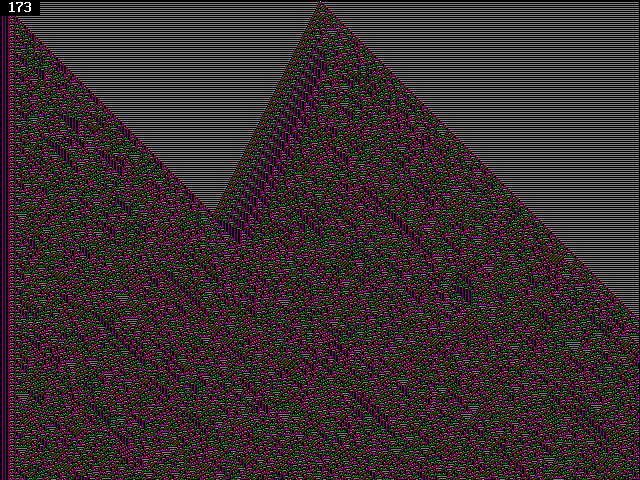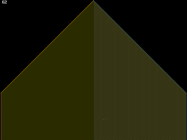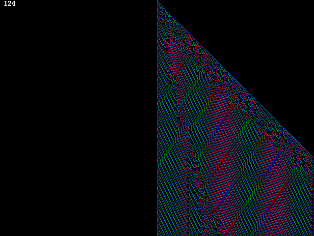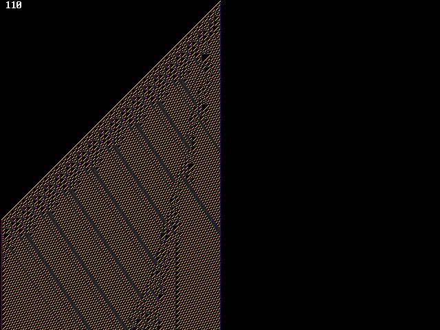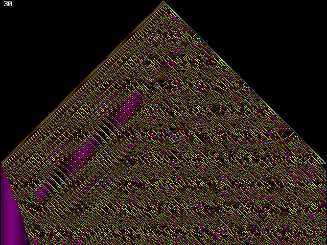These programs were based off of reading New Kind of Science, A - Stephen Wolfram - Wolfram Media which covers cellular automata. While reading the book it seemed that it would be interesting not only to see the cellular automata work on something other than the printed page, but to learn more detail by becoming familiar with algorithms that can generate these patterns. Ideally this would be carried out graphically. The end result was an entire suite of programs that progressed from an initial 'experiment' with the idea into more details. meanwhile tuning the logic for speed and best graphical representation. The programs were written in BASIC which was then compiled into EXE files. These BASIC files would run the monitor in a CGA graphics mode and draw the CA(cellular automata) on the screen pixel by pixel. Below are some screenshots of the outputs for a few of the more interesting CA 8-bit rule (0-255)diagrams. This shows a progression from simple, patterned, fractal, mixed pattern/chaos and finally chaotic. The thumbnails are a bit distorted due to re-sizing, click on them for a larger cleaner 640 x 480 view.            CA basically exhibits a few types of behavior. It can have the following behavior and the programs draw graphical representations of it. It can dead end and do nothing. Some cases don't go anywhere, nothing happens past the initial seed pixel which is intentional put on the screen. It can draw a straight or angled one dimensional line off of the initial seed pixel. It can fill the screen either with one solid color or a pattern such as alternating lines. It can produce a filled area of additive growth, such as a filled triangle that extends off of the seed pixel. It can produce regular and nested fractal patterns, which usually contain triangular forms. Finally it can produce, most surprising, chaos, patterns that look quite random but seem to have islands of order within them. I am not going to go into the details of CA here for a deeper look go to Stephen Wolfram A New Kind of Science where the entire text is available on line. For more one chaos theory material on this site see the Recursive Logistic Equation Page. The basic concept uses AND/OR type of logic and a 8 bit bitmap to decide what color a pixel will become in a particular row and column based on values in the row before it at the positions directly above, above and to the left and above and to the right. The decisions made are based on a rule number. For example rule 0 = 00000000 results in a non-operation, no matter what the previous row had for the state of the pixel directly above and left/ right, the new pixel will be blank. The rule 255 = 11111111 will turn on the new pixel no matter what the state of the pixel directly above and left/ right. In between there are a bunch of different rules that respond by say turning on the new pixel when the pixel above it is on but the ones above it to the left and right are not on for example. Which would be rule 64 (0100000). The BASIC code for the pixel operations is as follows. 230 if point(x-1,y) <> 15 and point(x,y) <> 15 and point(x+1,y) <> 15 then pset(x,y+1),a[7] 240 if point(x-1,y) <> 15 and point(x,y) <> 15 and point(x+1,y) = 15 then pset(x,y+1),a[6] 250 if point(x-1,y) <> 15 and point(x,y) = 15 and point(x+1,y) <> 15 then pset(x,y+1),a[5] 260 if point(x-1,y) <> 15 and point(x,y) = 15 and point(x+1,y) = 15 then pset(x,y+1),a[4] 270 if point(x-1,y) = 15 and point(x,y) <> 15 and point(x+1,y) <> 15 then pset(x,y+1),a[3] 280 if point(x-1,y) = 15 and point(x,y) <> 15 and point(x+1,y) = 15 then pset(x,y+1),a[2] 290 if point(x-1,y) = 15 and point(x,y) = 15 and point(x+1,y) <> 15 then pset(x,y+1),a[1] 300 if point(x-1,y) = 15 and point(x,y) = 15 and point(x+1,y) = 15 then pset(x,y+1),a[0] The function point returns TRUE or FALSE based on whether or not the pixel in that location contains the value 15, which is white in CGA, 4 bit color. Black corresponds to 0. Based on the logic <> ( not equal) or = (equal) plus anding the previous left, right and center pixels the new pixel in the row below the old is set using the pset function. The pset sets the pixel to color value a[0...7], the array a is encoded with the rule. What this means is that for let's say rule zero a[0] to a[7] are set to zero for black. So no matter what happens a black pixel is generated. As you can image if the rule turns the pixel black no matter what the CA will die out. The inverse case of 255 sets all of a[0] to a[7] 15 white, which floods the screen with white. The truth table for the rule number versus the logic used to represent it is as follows. Rule LCR 128 000 64 001 32 010 16 011 8 100 4 101 2 110 1 111 L represents Left, C center and R right for the pixels(cells) above the pixel that needs to be drawn. The logic is such that the values shown yield a true. For instance rule 128 would mean Left pixel white = FALSE and Center pixel white = FALSE and Right pixel white = FALSE means paint new pixel with. Obviously the rules can be compounded to yield all the values from 0 - 255. For example rule 30 means apply 16+8+4+2 = 30, so apply the ones listed (16,8,4,2) in the truth table together. Thirty would be 011 AND 100 AND 101 AND 110. Later versions of the programs used coding schemes for color so that the pixels were not just black and white but a shade of color depending on which part of the logic was being applied. This was done by loading the array a with values in terms of CGA color in the color handler subroutine. Looking at the code itself is the best way to understand it. 'color handler 1000 if n = 7 then a[n] = 0 '!RGB = blk 1001 if n = 6 then a[n] = 1 'XXB = blue 1002 if n = 5 then a[n] = 2 'XGX 1003 if n = 4 then a[n] = 3 'XGB = torq 1004 if n = 3 then a[n] = 4 'RXX 1005 if n = 2 then a[n] = 5 'RXB = pur 1006 if n = 1 then a[n] = 14 'RGX = yel 1007 if n = 0 then a[n] = 8 ' RGB but not, use gray 1008 return Where n is the number of the array position for the corresponding line of the rule in the truth table (think 128 = 2^7), n is the exponent in terms of powers of 2. The color runs from black to gray, gray chosen instead of white to yield a higher color contrast. !RGB means black, with RGB ( Red/Green/Blue) turned off. XXB means turn CGA blue on a value of 1. XGB means green and blue ON for torquise, a value of 3 and so on. This is the core functionality of the programs. Other than the logic above the initialization section converted the rule entered by the user 0-255 to the binary pattern of the rule which loads the color into the array a. From this point there is a nested looping that runs from 0-640 for the X direction and 0 - 480 for the Y direction. The loops are such that the X incrementing loop is inside of the Y loop. The program effectively scans each horizontal line pixel by pixel and performs a return at the end to the next row in the Y direction. In order to start off somewhere an initial seed pixel or pixels is needed in the first row. In the code there is an initialization that writes one white pixel in the center of the first row. I have also tried to put multiple initial pixels and patterns of them, this makes for interesting graphics as the multiple CA diagrams crash, merge or bounce off of one another. One of the most interesting ones looks like the migration of a fatigue crack in a solid material. For more on this topic on this site see CAFL Control Algorithm Back to Top   CAT Transceiver control program This program is used to control the Yaseu HF Transceiver CAT serial link. I am using a FT767GX in particular. The code is written in C. The transceiver has a serial port that operates at 4800 baud. The program was written over the Winter 2005-06, when there wasn't much else going on. The depths of winter become a hibernation mode time, a perfect time for indoor projects like these. The protocol followed while writing this program was not to try connect right away with the transceiver. Trying to write a program to control the transceiver and using it would be flying blind. I already had written a terminal program to allow 2 PC's to connect using the serial port. The core of this program was built on to create the CAT control program by a first sending a basic message and looking for the echo and then sending the acknowledge. Another program was then written from this that simulated what the transceiver would be doing during the exchange of messages. The transceiver simulator put what it received on the serial bus on the screen and then echoed back the commands to the main program, which in return displayed this on the screen and returned an acknowledge when there was a match. Using the main CAT control program and a simulation program for the transceiver and linking the 2 pc's in my office together serially made the debugging go fast. Once a few basic messages went through OK it was time to concentrate on decode the status messages shown below (Figure 2). Once a few basic 5 byte status messages decoded fine it was time to complete the program. This basically meant handling every command in the list. At first I just tried out turning the CAT control off and on and adjusting frequency, now I filled in the blanks for all of the rest of the messaging. Once the program could send all of the commands and receive 5 byte status blocks back from the transceiver simulator, I tried it out on the real transceiver. It was time to solder up an adapter cable and let it run. From the very beginning the transceiver would respond correctly to the commands sent by the PC. The PC was glitching on the echo and the status blocks and I had temporarily set things up to unconditionally send an acknowledge to the transceiver. I confirmed that part of it worked. The processor in the transceiver which is circa 1987 runs slow, it takes time to react to the commands that come across the serial line. All I needed to put into the program was a 5ms delay between messages and all of it worked fine. I finished up by writing the code to handle all 86 bytes of the status message. This was once again done using the transceiver simulator program to play against the main CAT control program for some of the cases. I did not test them all with the simulator because there was a lot of redundancy in the status message. Eventually it all worked well and I went on to write some DOS batch files that can execute the CAT control program automatically. There is even a feature to active certain controls based on the time of day, so the transceiver can change controls on a schedule through the batch file as well. Below is the entire setup and a screenshot of a message transaction. 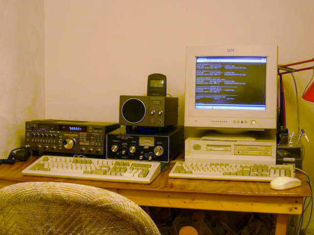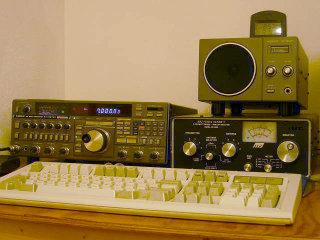The CAT control light comes on when the transceiver is under remote control. 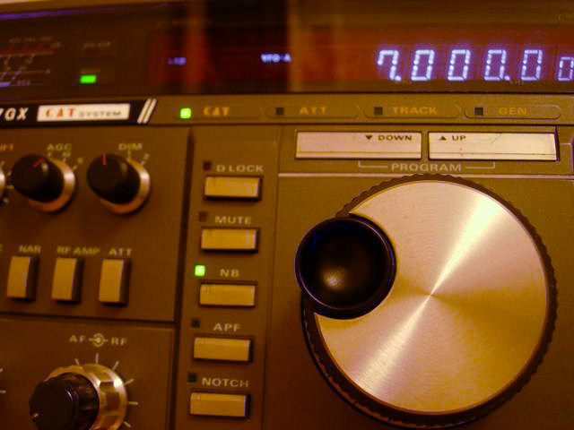The screen on the PC showing CAT commands being executed. In the first the commandcat modesel am is being executed. This sets the mode to AM. In the second the command cat vfomr vfoa followed by cat vfomr vfob is sent. This command swaps between the two variable frequency oscillators in the transceiver. The frequency switches to 10MHz and then back to 7MHz. The command structure for controlling the transceiver is fairly simple. The following is an example of the transaction across the serial bus for the command that would be entered as cat fset 1425000. Protocol: 4800-1-8-2-N Ex: FSET 1425000 (14.25000) |01|42|50|00|FSET ... becomes... CMD Block = 0x00|0x50|0x42|0x01|0x08 LSD MSD Transaction: SI ------|0x00|0x50|0x42|0x01|0x08|--------------------------|0x??|xx|xx|xx|xx|------------------ command ACK SO --------------------------------|0x00|0x50|0x42|0x01|0x08|------------------|SB|0x01|42|50|00| echo 5-byte Status(5-86 is poss.) (5ms gaps between SO and SI's.) The following image is a screenshot of cat fset 009690, setting the frequency to 9.69MHz. Yaesu provides all of the information in the manual that allows you to build code to control the transceiver. As you can see in the example above. First a command is sent, the transceiver then echoes this back, acknowledge is sent back to the transceiver, then transceiver then processes the command, then the transceiver sends back a variable length status. In the status SB is the leading status byte which is interpreted as follows. Status Byte(SB) BIT 7 CAT 1 = ON 6 CLAR 1 = ON 5 MR 1 = ON 4 VFO A/B 1 = VFO B 3 SPLIT 1 = ON 2 Tx Inhib 1 = ON 1 H/G 1 = G 0 PTT 1 = TX The following is the list of commands that are possible, I kept with the syntax used by Yaesu. In other words CATSW in there list is sent out as cat catsw on by the program. COMMANDS (Hex)MSD (BCD) LSD Instr CMD D1 D2 D3 D4 Remarks Status Size ------------------------------------------------------------------------------------------------- CATSW 00 P1 XX XX XX p1 value: OO=ON. 01=OFF 86 CHECK 01 xx xx xx xx No op: return status Only 86 UP10Hz 02 xx xx xx xx Step frequency UP 10 Hz 5 DN10Hz 03 xx xx xx xx Step frequencv down 10 Hz 5 PRGUP 04 p1 p2 xx xx p1 & p2 * 5 PRGDN 05 p1 p2 xx xx p1 & p2 * 5 BANDUP 06 xx xx xx xx Step UP one Band** 5 BANDDN 07 xx xx xx xx Step down one Band** 5 FSET 08 p1 p2 p3 p4 Frequency Set (see EXAMPLE) 5 VFOMR 09 p1 xx xx xx VFO/Memory Select: p1 value: 00=VFO A,01 =VFO B, 02=MR 5 MEMSEL 0A p1 xx xx xx p1 value = memorv no.(0 -9) 8 MODESEL 0A p1 xx xx xx p1 value: 10h=LSB, 11h=USB,12h=CW.13h=AM 14h=FM,15h=FSK 8 HGSEL 0A p1 xx xx xx p1 value: 20h=HAM 21h=GEN 26 SPLITOG 0A 30h xx xx xx Toggles SPLIT on/off 26 CLARTOG 0A 40h xx xx xx Toggles Clarifier on/off 26 MTOV 0A 50h xx xx xx Memory to VFO 26 VTOM 0A 60h xx xx xx VFO to Memory 86 SWAP 0A 70h xx xx xx Swap VFO and Memory 5 ACLR 0A 80h xx xx xx Turn off SPLIT. CLAR. OFFSET 5 TONESET 0C p1 p2 p3 xx p1,p2 = Tone Freq(BCD) *** p3=00 for Low-Q 01 for Hi-Q 5 ACK 0b xx xx xx xx Required after each Code no echo ------------------------------------------------------------------------------------------------- xx = any value: byte will be echoed, but will not affect command function. * 00 00 to 99 99 representing 0 to 99.99 kHz (BCD) . ** Band'steps determined by current Ham/Gen selection: Ham bands, or 0.5 MHz. *** 06 70 to 25 03 representing 67.0 to 250.3 Hz (BCD). See Tone Table 3 for list of valid tone frequencies. Figure 2, the typos in this are not mine. The OCR from the bed scanner had trouble with reading this out of the FT767 manual. Byte Contents Rer. No. Table 1 Status Flaas . 1 2-5 Oneratina Freauencv (BCD) 2 6 Selected CTCSS Tone 3 7 Selected Mode 4 8 Selected Memorv Channel No. (0- 9) 9-12 Clarifier Freauencv (BCD) 2 13 Clarifier CTCSS Tone* 3 14 Clarifier Mode 4 15-18 VFO A FreQuencv (BCD) 2 19 VFO A CTCSS Tone* 3 20 VFO A Mode 4 21-24 VFO B Freauencv (BCD).. 2 25 VFO B CTCSS Tone* 3 26 VFO B Mode 4 27-30 Memorv Channel 0 Freahencv (BCD) 2 31 Memorv Channel 0 CTCSS Tone* 3 32 Memorv Channel 0 Mode 4 33-38 Memorv Ch 1 (same format as 27-32)** 39-44 Memorv Ch 2 (same format as 27-32)** 45-50 Memorv Ch 3 (same format as 27-32)** 51-56 Memorv Ch 4 (same format as 27-32)** 57-62 Memorv Ch 5 (same format as 27-32)** 63-6s.. Memorv Ch 6 (same format as 27-32)** 69-74 Memorv Ch 7 (same format as 27-32)** 75-80 Memorv Ch 8 (same format as 27-32)** R1-RF; Mpmnru ('10 Q The following screenshot is a status dump that occurs when cat catsw on is sent. Debug mode- The CAT control program provides a debug mode for both the CAT.exe control program and the cattest.exe simulator program. When either program is called with the /d argument, debugging output is provided. This is mostly for the development of the program, in the case of the CAT program itself it can be used to troubleshoot the serial connection to and from the transceiver. The following are a few screenshots of the CAT control program ran with debug output The first is setting the frequency in debug mode, the second is setting the modulation type to USB( upper side band) and the third is a tweak the frequency up 10 Hz command. By setting the frequency to 012345 which translates into 12.34500 MHz it is obvious from the debug data what is going on. The command for FSET is 8, the 10's and 100's Hertz are set to 0. So the command out is 0|45|23|1|8, CAT always sends things out 'backwards' and each byte sent out is a type of BCD-HEX format that goes as high as 99. The transceiver echoes back 0|45|23|1|8 to the CAT program. The CAT program reechoes the frequency and 0xb which is the ack upon which the transceiver changes the frequency to 12.34500. Then the transceiver sends out a 5 byte status to the CAT program. The status of 0|45|23|1|80. The status contains the frequency and 0x80 which is a bit map of flags, in this case with bit 7 set. Looking at the table below the status tells that CAT is ON, in control of the radio, VFO is A H/G(HAM/GENERAL COVERAGE) is set to H (HAM) and PTT Status Byte(SB) BIT 7 CAT 1 = ON 6 CLAR 1 = ON 5 MR 1 = ON 4 VFO A/B 1 = VFO B 3 SPLIT 1 = ON 2 Tx Inhib 1 = ON 1 H/G 1 = G 0 PTT 1 = TX Back to Top   Software Portfolio I am keeping a list of software that I have written for reference and for anyone that is interesting in more detail. Software Portfolio Back to Top   Original Build Date:12-2-2000 Last updated 3-15-2010