The files that the Digital File Processing (DFP) software I wrote work on, are Wave audio files that were created by recording with a SoundBlaster Card. The SoundBlaster operates using an onboard digital to analog and analog to digital converter as the main onboard workhorses with additional DSP hardware on-board. External connections are available for audio input and output. Internally the SoundBlaster is addressable through software where the data stream in 8 bit or 16 bit (for this model)can be retrieved or stored in files. I tested the input of the SoundBlaster auxiliary input jack with a power supply and found that it can be faked into being almost DC coupled (Freq. response <0.0001Hz) through using a high resistance (>1M) in series. Care must be exercised not to overvoltage or overcurrent the input. I used a voltage divider with 100X division. The device is capable of input a few volts positive and negative and also output in that range. Therefore the device could in principle be used as a voltmeter, scope, spectrum analyzer and arbitrary waveform signal generator.

The Wave files created by the SoundBlaster consist of a header followed by the data corresponding to the signal level. With an 8bit file the 0 volt reading generally falls at 128 or 127 (80h or 7Fh), allowing the positive excursion to reach 255 (FFh)and negative excursion to reach 0. The following is a file dump of a recording of a positive and negative delta function followed by zero input.

-d

1277:0100  52 49 46 46 38 2B 00 00-57 41 56 45 66 6D 74 20   RIFF8+..WAVEfmt 
1277:0110  12 00 00 00 01 00 01 00-22 56 00 00 22 56 00 00   ........"V.."V..
1277:0120  01 00 08 00 00 00 64 61-74 61 11 2B 00 00 80 7F   ......data.+....
1277:0130  7F 80 80 80 00 80 80 80-80 80 80 80 80 80 80 80   ................
1277:0140  FF 80 80 80 80 80 80 80-80 80 80 80 80 80 80 80   ................
1277:0150  00 80 80 80 80 80 80 80-80 80 80 80 80 80 80 80   ................
1277:0160  80 80 80 80 80 80 80 80-80 80 80 80 80 80 80 80   ................
1277:0170  80 80 80 80 80 80 80 80-80 80 80 80 80 80 80 80   ................
-d<
1277:0180  80 80 80 80 80 80 80 80-80 80 80 80 80 80 80 80   ................
1277:0190  80 80 80 80 80 80 80 80-80 80 80 80 80 80 80 80   ................
1277:01A0  80 80 80 80 80 80 80 80-80 80 80 80 80 80 80 80   ................
1277:01B0  80 80 80 80 80 80 80 80-80 80 80 80 80 80 80 80   ................
1277:01C0  80 80 80 80 80 80 80 80-80 80 80 80 80 80 80 80   ................
1277:01D0  80 80 80 80 80 80 80 80-80 80 80 80 80 80 80 80   ................
1277:01E0  80 80 80 80 80 80 80 80-80 80 80 80 80 80 80 80   ................
1277:01F0  80 80 80 80 80 80 80 80-80 80 80 80 80 80 80 80   ................

-q

The delta functions can be seen as the frst byte of FF after 1277:0140 and 00 after 1277:0150. The header is 52 bytes long at the top and contains information which designations the characteristics of the file.

For example the fact that this file is sampled at 22kHz using 8 bits and is monaural is stored there.

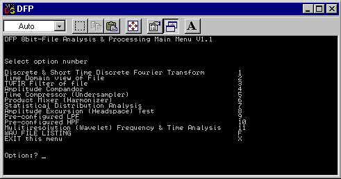
Editors are available to cut and paste these files using a time domain graph of the file. Standard features of these editors also include volume control, file reversal, mixing files, inverting waveforms, echos, fades, mixing two files and file format conversion, all time domain editing functions. Some editors can filter files using an available graphic equalizer. But, in general there is a lack of features for handling the frequency domain manipulation of files.

This is the focus of this software which allows for viewing and manipulation of the files in the frequency domain. To view the files in the frequency domain the files are read in binary form (skipping over the 52 byte header as with all of the software in this package) and a discrete Fourier Transform is calculated . A specified number of samples is read in depending on the number inputted. One half of this number is taken as the Nyquist folding frequency. There is an outer loop in the code that runs from 0 to the folding frequency. In this loop a delta change in angle of 2pi multiplied by the index and divided by the number of samples is calculated. The inner loop summations and the angle variable are cleared in the outer loop.The inner loop runs from 0 to the number of samples minus 1. In the inner loop summations are taken in the imaginary and real axes of the indexed sample value multiplied by the sine and cosine of the angle values. While in the inner loop the angle is incremented by the delta value with every pass. These summations values are held in an array. Later on in the program the absolute value of the summations is taken and plotted against a frequency axis.

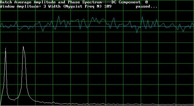
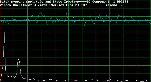
The spectral analysis program also allows for taking multiple batches of Short Time Fourier Transform samples from a file and forming the average of these amplitude values. This allows a amplitude -v- frequency plot of a signal which has much variation in the time domain. As for a white noise frequency response test of a system, the more batches averaged yields a frequency response which approaches a true response. Zoom functions are also incorporated in this software module. Data is outputted to a *.DFT file which consists of a frequency index followed by amplitude and phase at that frequency, suitable for spreadsheet import.

In the software package there are two filters a transversal FIR and IIR. These both can take user inputted A and B coefficients. Both programs contain a loop which inputs binary data from the wave file and applies multiplication with the coefficients to the (X-n in for FIR)data or (Y-n in for IIR)and collects the summation. This summation (Y out) is the written back to the file as the program moves down the file, much like an "assembly line". Both filter programs can be applied in succession to create a combination filter to represent any arbitrary transfer function.

Also in the package is a compandor. This is a simple type of compandor which takes input from the binary file and multiplies it with user inputted linear factor (volume control) and raises it to a power. Then the new value is written back into the file, until the end is reached. For example inputting 0.5 (square root) compresses the amplitude, followed with 2 (squared) expands the amplitude back to the original. Effects of artificial non-linear devices can also be created with method.

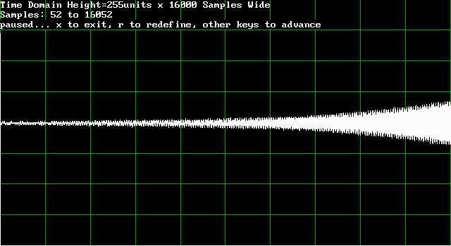
A viewer is available for the time domain representation of the file. This program reads in the file data and plots the stored amplitude values versus a given number of samples, which is adjustable. The viewer can step through the file and allows a rescan of any section to be made in greater or lesser detail, providing zoom functions. The final frame on the screen when the program is exited is captured to a *.TD file, which contains sample numbers and the corresponding amplitude, suitable for spreadsheet import. (8/1/1999)

Additional features described below have been added since the document above has been written.